Comparision: FEM vs. other methods

In this section, we compare the performance of Free Energy Minimization (FEM) method with other existing methods based on mean field approximations and Maximum Likelihood Estimation (MLE). We shall show that FEM is more accurate than other methods. Additionally, FEM is computationally much faster than MLE.

First of all, we import the necessary packages to the jupyter notebook:

import numpy as np
import sys
import timeit
import matplotlib.pyplot as plt
import simulate
import inference
%matplotlib inline

np.random.seed(1)

We generate a true interaction matrix w0 and time series data s0.

# parameter setting:
n0 = 40  # number of variables
g = 4.0  # interaction variability parameter

w0 = np.random.normal(0.0,g/np.sqrt(n0),size=(n0,n0))

# generating time-series data
l = int(4*(n0**2))
s0 = simulate.generate_data(w0,l)

Suppose only a subset s of variables is observed.

nh0 = 15
n = n0 - nh0
s = s0[:,:n].copy()

Suppose first that we know the number of hidden variables so we set nh to its actual value.

nh = nh0

Let us write a plot function to compare actual couplings and inferred couplings.

def plot_result(w0,w):
    plt.figure(figsize=(13.2,3.2))

    plt.subplot2grid((1,4),(0,0))
    plt.title('observed to observed')
    plt.plot([-2.5,2.5],[-2.5,2.5],'r--')
    plt.scatter(w0[:n,:n],w[:n,:n])
    plt.xticks([-2,0,2])
    plt.yticks([-2,0,2])
    plt.xlabel('actual interactions')
    plt.ylabel('inferred interactions')

    plt.subplot2grid((1,4),(0,1))
    plt.title('hidden to observed')
    plt.plot([-2.5,2.5],[-2.5,2.5],'r--')
    plt.scatter(w0[:n,n:],w[:n,n:])
    plt.xticks([-2,0,2])
    plt.yticks([-2,0,2])
    plt.xlabel('actual interactions')
    plt.ylabel('inferred interactions')

    plt.subplot2grid((1,4),(0,2))
    plt.title('observed to hidden')
    plt.plot([-2.5,2.5],[-2.5,2.5],'r--')
    plt.xticks([-2,0,2])
    plt.yticks([-2,0,2])
    plt.scatter(w0[n:,:n],w[n:,:n])
    plt.xlabel('actual interactions')
    plt.ylabel('inferred interactions')

    plt.subplot2grid((1,4),(0,3))
    plt.title('hidden to hidden')
    plt.plot([-2.5,2.5],[-2.5,2.5],'r--')
    plt.scatter(w0[n:,n:],w[n:,n:])
    plt.xticks([-2,0,2])
    plt.yticks([-2,0,2])
    plt.xlabel('actual interactions')
    plt.ylabel('inferred interactions')

    plt.tight_layout(h_pad=1, w_pad=1.5)
    plt.show()

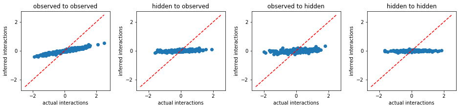
Naive Mean-Field approximation

print('nMF:')
cost_obs,w,sh = inference.infer_hidden(s,nh,method='nmf')
w,sh = inference.hidden_coordinate(w0,s0,w,sh)
plot_result(w0,w)

nMF:

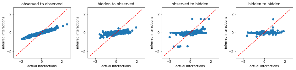
Thouless-Anderson-Palmer mean field approximation

print('TAP:')
cost_obs,w,sh = inference.infer_hidden(s,nh,method='tap')
w,sh = inference.hidden_coordinate(w0,s0,w,sh)
plot_result(w0,w)

TAP:

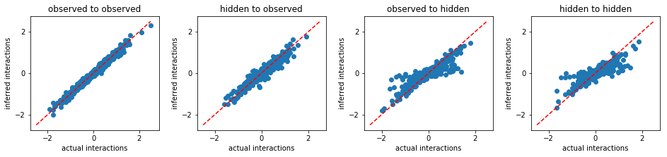
Exact mean field approximation

print('eMF:')
cost_obs,w,sh = inference.infer_hidden(s,nh,method='emf')
w,sh = inference.hidden_coordinate(w0,s0,w,sh)
plot_result(w0,w)

eMF:

Maximum Likelihood Estimation

print('MLE:')

start_time = timeit.default_timer()

cost_obs,w,sh = inference.infer_hidden(s,nh,method='mle')
w,sh = inference.hidden_coordinate(w0,s0,w,sh)

stop_time=timeit.default_timer()
run_time=stop_time-start_time
print('run_time:',run_time)

plot_result(w0,w)

MLE:
('run_time:', 9970.889276981354)

Free Energy Minimization

print('FEM:')

start_time = timeit.default_timer()

cost_obs,w,sh = inference.infer_hidden(s,nh,method='fem')
w,sh = inference.hidden_coordinate(w0,s0,w,sh)

stop_time=timeit.default_timer()
run_time=stop_time-start_time
print('run_time:',run_time)

plot_result(w0,w)

FEM:
('run_time:', 515.2393028736115)

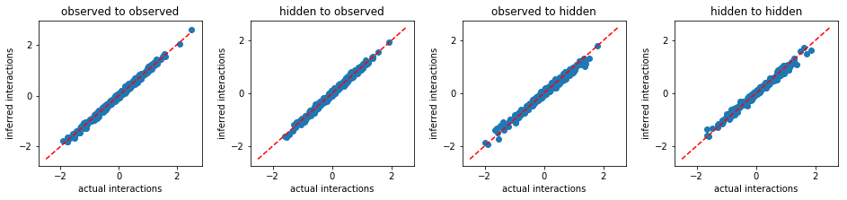
From the above results, we conclude that FEM outperforms other existing methods. Beside more accurate inference, FEM works much faster than MLE. For instance, to solve the same problem, FEM took only 515 seconds, however, MLE took 9970 seconds.