Results

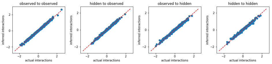
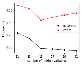
We demonstrate the performance of our method in analyzing binary data generated from the kinetic Ising model simulations in the following. Using configurations of a subset of variables, we will recover the interactions (including observed to observed, hidden to observed, observed to hidden, and hidden to hidden), the configurations of hidden variables, and the number of hidden variables.

First of all, we import the necessary packages to the jupyter notebook:

import numpy as np
import sys
import matplotlib.pyplot as plt
import simulate
import inference
%matplotlib inline

np.random.seed(1)

We consider a system of n0 variables interacting each others with interaction variability parameter g.

# parameter setting:
n0 = 40  # number of variables
g = 4.0  # interaction variability parameter

w0 = np.random.normal(0.0,g/np.sqrt(n0),size=(n0,n0))

Using the function simulate.generate_data, we then generate a time series of variable states according to the kinetic Ising model with a data length l.

l = int(4*(n0**2))

s0 = simulate.generate_data(w0,l)

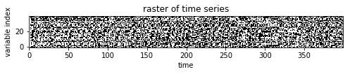
A raster of variable configurations s0 is plotted:

plt.figure(figsize=(8,6))
plt.title('raster of time series')
plt.imshow(s0.T[:,:400],cmap='gray',origin='lower')
plt.xlabel('time')
plt.ylabel('variable index')
plt.show()

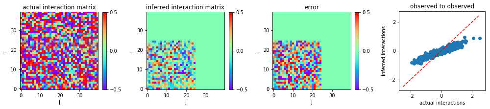
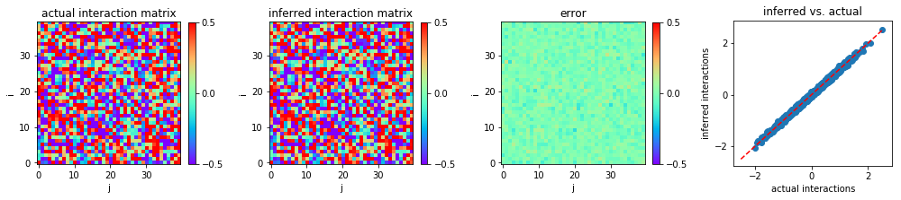
Using the configurations of entire system s0, we can infer sucessfully the interactions between variables:

w = inference.er(s0)

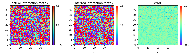
We plot the heat map of the actual interaction matrix w0, the inferred interaction matrix w, and the error in inference, i.e., the discrepancy between w0 and w.

plt.figure(figsize=(14,3.2))

plt.subplot2grid((1,4),(0,0))
plt.title('actual interaction matrix')
plt.imshow(w0,cmap='rainbow',origin='lower')
plt.xlabel('j')
plt.ylabel('i')
plt.clim(-0.5,0.5)
plt.colorbar(fraction=0.045, pad=0.05,ticks=[-0.5,0,0.5])

plt.subplot2grid((1,4),(0,1))
plt.title('inferred interaction matrix')
plt.imshow(w,cmap='rainbow',origin='lower')
plt.xlabel('j')
plt.ylabel('i')
plt.clim(-0.5,0.5)
plt.colorbar(fraction=0.045, pad=0.05,ticks=[-0.5,0,0.5])

plt.subplot2grid((1,4),(0,2))
plt.title('error')
plt.imshow(w0-w,cmap='rainbow',origin='lower')
plt.xlabel('j')
plt.ylabel('i')
plt.clim(-0.5,0.5)
plt.colorbar(fraction=0.045, pad=0.05,ticks=[-0.5,0,0.5])

plt.subplot2grid((1,4),(0,3))
plt.title('inferred vs. actual')
plt.plot([-2.5,2.5],[-2.5,2.5],'r--')
plt.scatter(w0,w)
plt.xticks([-2,0,2])
plt.yticks([-2,0,2])
plt.xlabel('actual interactions')
plt.ylabel('inferred interactions')

plt.tight_layout(h_pad=1, w_pad=1.5)
plt.show()

However, in the real world, it is likely that we do not observe the entire system, but only a subset of variables. For instance, suppose that there are nh0 hidden variables, so the number of observed variables is n = n0 - nh0 and the observed configurations are s = s0[:,:n].

nh0 = 15
n = n0 - nh0
s = s0[:,:n].copy()

Ignoring hidden variables

Let us see what happen if we ignore the existence of hidden variables and infer the interactions between the observed variables. Using observed configurations s, we can try to infer interactions between the observed variables:

w = inference.er(s)

The heat map of the actual interaction matrix w0, the inferred interaction matrix w (only from observed to observed), and the error between them are plotted.

w_infer = np.zeros((n0,n0))
w_infer[:n,:n] = w

error = np.zeros((n0,n0))
error[:n,:n] = w0[:n,:n] - w

#-------------------------------------
plt.figure(figsize=(14,3.2))

plt.subplot2grid((1,4),(0,0))
plt.title('actual interaction matrix')
plt.imshow(w0,cmap='rainbow',origin='lower')
plt.xlabel('j')
plt.ylabel('i')
plt.clim(-0.5,0.5)
plt.colorbar(fraction=0.045, pad=0.05,ticks=[-0.5,0,0.5])

plt.subplot2grid((1,4),(0,1))
plt.title('inferred interaction matrix')
plt.imshow(w_infer,cmap='rainbow',origin='lower')
plt.xlabel('j')
plt.ylabel('i')
plt.clim(-0.5,0.5)
plt.colorbar(fraction=0.045, pad=0.05,ticks=[-0.5,0,0.5])

plt.subplot2grid((1,4),(0,2))
plt.title('error')
plt.imshow(error,cmap='rainbow',origin='lower')
plt.xlabel('j')
plt.ylabel('i')
plt.clim(-0.5,0.5)
plt.colorbar(fraction=0.045, pad=0.05,ticks=[-0.5,0,0.5])

plt.subplot2grid((1,4),(0,3))
plt.title('observed to observed')
plt.plot([-2.5,2.5],[-2.5,2.5],'r--')
plt.scatter(w0[:n,:n],w_infer[:n,:n])
plt.xticks([-2,0,2])
plt.yticks([-2,0,2])
plt.xlabel('actual interactions')
plt.ylabel('inferred interactions')

plt.tight_layout(h_pad=1, w_pad=1.5)
plt.show()

As expected, ignoring hidden variables leads to poor coupling inference.

In the following, we will take into account the existence of hidden variables.

Including hidden variables

Inferring interactions

We first assume that the number of hidden variables is known, nh = nh0. The interactions are then inferred by using the function inference.infer_hidden.

nh = nh0

cost_obs,w,sh = inference.infer_hidden(s,nh,method='er')

To compare the inferred interactions with the actual interactions, we use the function inference.hidden_coordinate to identify which inferred hidden variable corresponding to which actual hidden variable.

w,sh = inference.hidden_coordinate(w0,s0,w,sh)

Now, we plot the the heat map of the actual interaction matrix w0, the inferred interaction matrix w (including observed to observed, hidden to observed, observed to hidden, and hidden to hidden), and the error between them.

plt.figure(figsize=(11,3.2))

plt.subplot2grid((1,3),(0,0))
plt.title('actual interaction matrix')
plt.imshow(w0,cmap='rainbow',origin='lower')
plt.xlabel('j')
plt.ylabel('i')
plt.clim(-0.5,0.5)
plt.colorbar(fraction=0.045, pad=0.05,ticks=[-0.5,0,0.5])

plt.subplot2grid((1,3),(0,1))
plt.title('inferred interaction matrix')
plt.imshow(w,cmap='rainbow',origin='lower')
plt.xlabel('j')
plt.ylabel('i')
plt.clim(-0.5,0.5)
plt.colorbar(fraction=0.045, pad=0.05,ticks=[-0.5,0,0.5])

plt.subplot2grid((1,3),(0,2))
plt.title('error')
plt.imshow(w0-w,cmap='rainbow',origin='lower')
plt.xlabel('j')
plt.ylabel('i')
plt.clim(-0.5,0.5)
plt.colorbar(fraction=0.045, pad=0.05,ticks=[-0.5,0,0.5])

plt.tight_layout(h_pad=1, w_pad=1.5)
plt.show()

plt.figure(figsize=(13.2,3.2))

plt.subplot2grid((1,4),(0,0))
plt.title('observed to observed')
plt.plot([-2.5,2.5],[-2.5,2.5],'r--')
plt.scatter(w0[:n,:n],w[:n,:n])
plt.xticks([-2,0,2])
plt.yticks([-2,0,2])
plt.xlabel('actual interactions')
plt.ylabel('inferred interactions')

plt.subplot2grid((1,4),(0,1))
plt.title('hidden to observed')
plt.plot([-2.5,2.5],[-2.5,2.5],'r--')
plt.scatter(w0[:n,n:],w[:n,n:])
plt.xticks([-2,0,2])
plt.yticks([-2,0,2])
plt.xlabel('actual interactions')
plt.ylabel('inferred interactions')

plt.subplot2grid((1,4),(0,2))
plt.title('observed to hidden')
plt.plot([-2.5,2.5],[-2.5,2.5],'r--')
plt.xticks([-2,0,2])
plt.yticks([-2,0,2])
plt.scatter(w0[n:,:n],w[n:,:n])
plt.xlabel('actual interactions')
plt.ylabel('inferred interactions')

plt.subplot2grid((1,4),(0,3))
plt.title('hidden to hidden')
plt.plot([-2.5,2.5],[-2.5,2.5],'r--')
plt.scatter(w0[n:,n:],w[n:,n:])
plt.xticks([-2,0,2])
plt.yticks([-2,0,2])
plt.xlabel('actual interactions')
plt.ylabel('inferred interactions')

plt.tight_layout(h_pad=1, w_pad=1.5)
plt.show()

So our method infers the interactions accurately, not only observed to observed, but also hidden to observed, observed to hidden, and hidden to hidden.

Inferring configurations of hidden variables

Our algorithm allows us to infer the configurations of hidden variables simultaneously with the interactions in the previous step. The accuracy of the inference is calculated as

accuracy = 1 - (np.abs(s0[:,n:]-sh)/2.).mean()
print('inference accuracy: %2.2f %%'%(accuracy*100))

inference accuracy: 95.85 %

Inferring number of hidden variables

In the above sections, we recovered the interactions and configurations of hidden variables by using the right number of hidden variables, nh= nh0. However, in the real world, the number of hidden variables may not be available. In the following, we apply our method for various number of hidden variables nh and compute the discrepancies of observed variables cost_obs and the entire system cost.

nh_list = [11,13,15,17,19,21]
nnh = len(nh_list)

def discrepancy(nh):
    return inference.infer_hidden(s,nh,method='er')[0]

import multiprocessing
nPC = min(nnh,multiprocessing.cpu_count())
pool = multiprocessing.Pool(processes=nPC)
cost_obs_list = pool.map(discrepancy,nh_list)
pool.close()

cost_obs = np.array([cost_obs_list[i][-1] for i in range(nnh)])
cost = np.array([cost_obs[i]*(1+float(nh_list[i])/n) for i in range(nnh)])

We plot the discrepancies of observed variables cost_obs and the entire system cost as a function of the number of hidden variables. The minimum of cost corresponds to the true number of hidden variables.

plt.figure(figsize=(4,3.2))

plt.plot(nh_list,cost_obs,'ko-',linewidth=1,markersize=4,label='observed')
plt.plot(nh_list,cost,'r^-',linewidth=1,markersize=4,label='entire')
plt.xticks(nh_list)
plt.xlabel('number of hidden variables')
plt.ylabel('Discepancy')
plt.legend()
plt.show()

So we can infer the number of hidden variables based on the minimum of cost.